Gas detectors auto-placed by Kryptos on a real offshore deck, in 1 minute 8 seconds
A step-by-step gas mapping of the Huldra cellar deck, 38 × 40 × 5 m, with two timed optimisation runs: 17 open path and point detectors in 1 minute 8 seconds, 22 point detectors only in 2 minutes 39 seconds.
12 min read
Placing gas detectors by hand is a slow loop. Put a detector down, check what it covers, move it, check again, and repeat for every detector on every deck.
Kryptos runs that loop for you. This guide does a full gas mapping of one real deck, step by step, and times the part that usually takes the longest: placing the detectors. We ran the optimisation twice on the same deck to meet the coverage targets (90% 1ooN and 80% 2ooN) and the below table shows the summary of the optimisation runs:
| Run | Detectors allowed | Detectors placed | Time | Time to find optimised position per detector |
|---|---|---|---|---|
| 1 | Open path and point | 17 | 1 min 8 s | 4.0 s |
| 2 | Point only | 22 | 2 min 39 s | 7.2 s |
The rest of this post shows how to set up the same run on your own plant, and what the timings mean.
The deck we used
The model is the Huldra platform, an open offshore model, imported straight from its Navisworks file. See Navisworks file import done in just about a minute for how it was brought in.
We mapped the cellar deck: the lowest process deck of the topside, packed with pumps, vessels, pipe racks and the walkways between them. It is a good test, because a cramped deck is where gas can collect and where detectors are hardest to place by eye.
| Size | |
|---|---|
| Length (X) | 38.18 m |
| Width (Y) | 39.62 m |
| Height (Z) | 4.7 m |
| Floor area | about 1,513 m² |
| Volume checked for gas | about 7,110 m³ |
In round numbers, a 38 × 40 × 5 m box. Every point inside that box is checked against every possible detector spot, so the optimiser is weighing thousands of places a detector could go, not a handful.
The settings for both runs:
- Gas: hydrocarbons (HC).
- Risk grade: Grade A over the whole deck.
- Gas cloud size: 10 m across. This is the smallest gas cloud the detectors must find. A cloud counts as found when it reaches a detector.
- Targets: 90% of the deck seen by at least one detector (1ooN) and 80% seen by at least two (2ooN).
- Detector heights: open path detectors 2 m to 5 m above the deck, point detectors 0.5 m to 1.5 m above it.
Step 1: Create the area
An area is the part of the plant you are mapping, usually one fire zone. Here, it is the cellar deck.
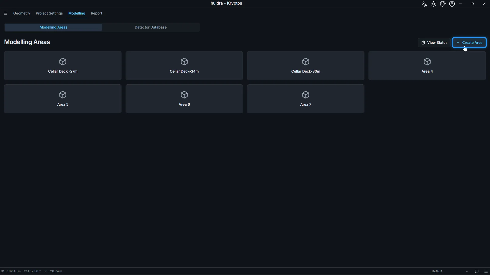
- Open the Modelling tab and click Create Area.
- The new area opens on Area Settings. Under Area Coordinates, enter the Min and Max of each axis, or drag the white handles in the 3D view.
For the cellar deck, X runs from 92.9 m to 131.08 m, Y from 274.78 m to 314.4 m, and Z from 24.08 m to 28.78 m. Kryptos shows the size this gives under the boxes: ΔX 38.18 m, ΔY 39.62 m, ΔZ 4.7 m.
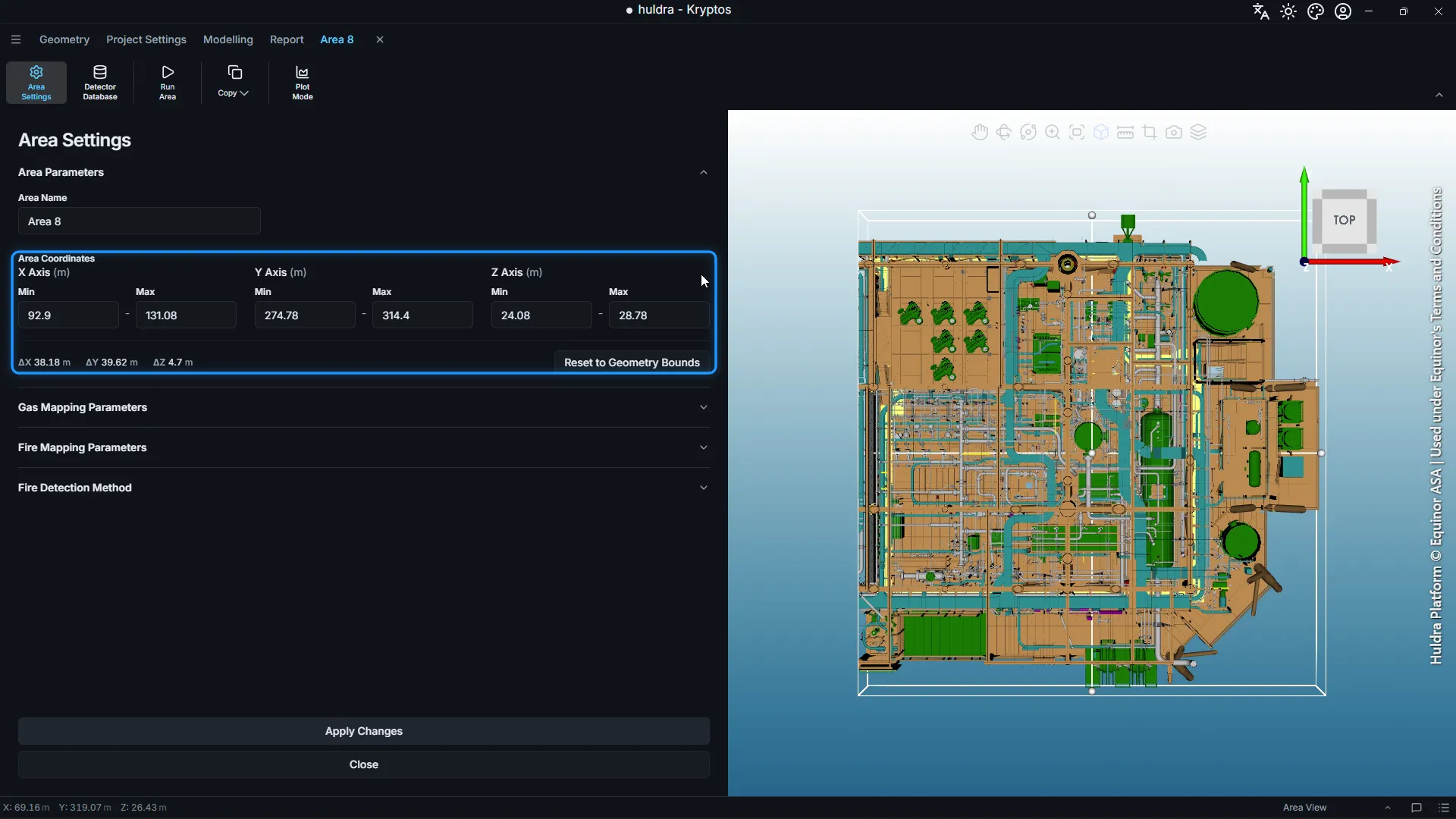
Tip: Keep the top of the area close to the top of the equipment. Every extra metre of height is more space to check, which makes the run slower and the plots harder to read. The cellar deck needs only 4.7 m.
In the screenshots, the area is called Area 8. Give yours a name people will recognise in the report, such as the deck name.
Step 2: Turn on the gas and set the cloud size
- Open Gas Mapping Parameters.
- Tick Enabled for each gas you need. We used HC (hydrocarbons).
- In the Grade A (m) box, enter the gas cloud size for that grade. We used 10.
- Click Apply Changes. The gas mapping is only created once you apply.
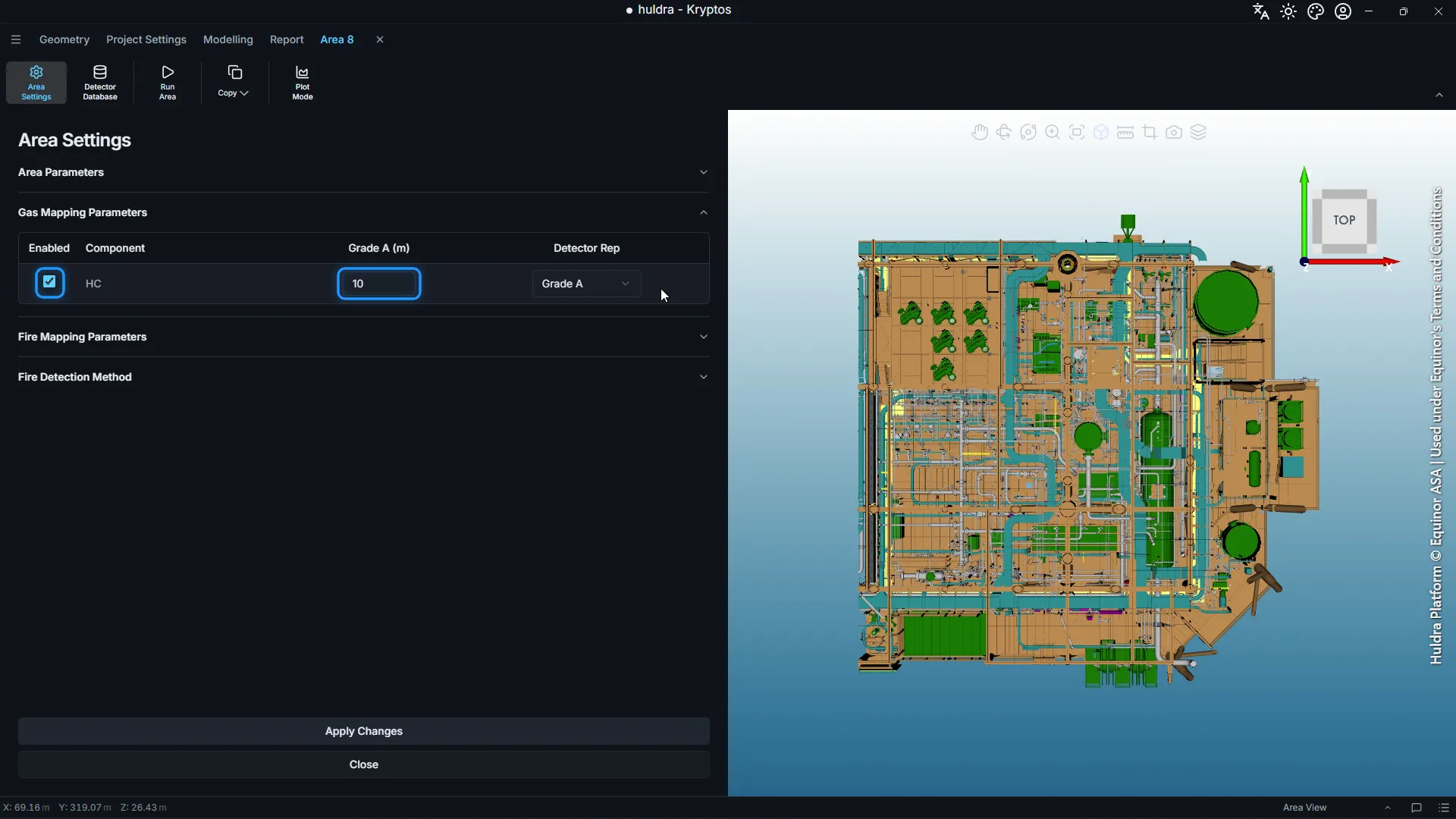
A smaller cloud is harder to find, so it needs more detectors. Use the cloud size your Fire & Gas philosophy sets for each grade.
Step 3: Draw the risk grade
A risk grade marks where a gas release could happen and how serious it would be. On the cellar deck, we drew one Grade A over the whole deck.
- In the area tree, select Risk Grade under Gas Mapping for HC, then click Add Grade.
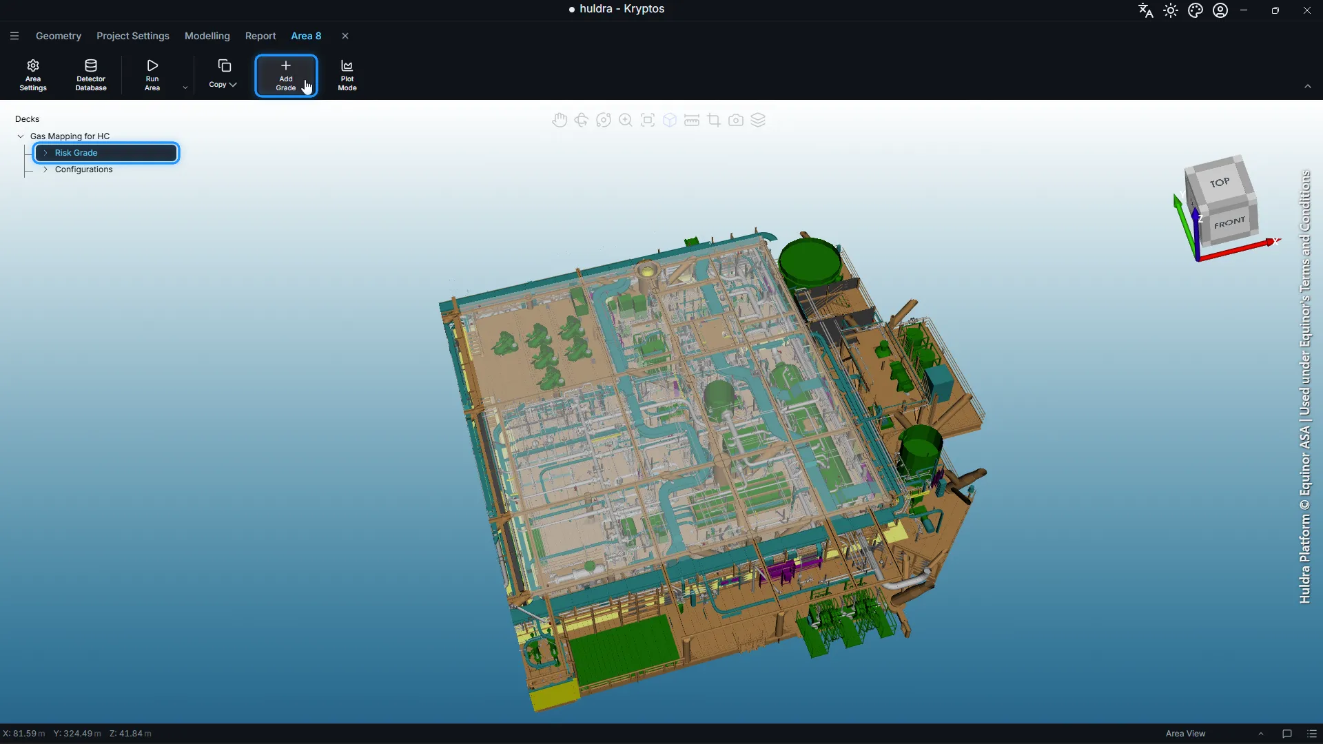
- Choose a Shape (Cubical, Cylindrical or Polygonal), a Draw Plane and the Extent, then click Draw Grade.
- Draw the outline in the 3D view and click Complete.
- Select the new grade in the tree and pick its Grade Type, such as Grade A.
Here is the grade being drawn over the cellar deck:
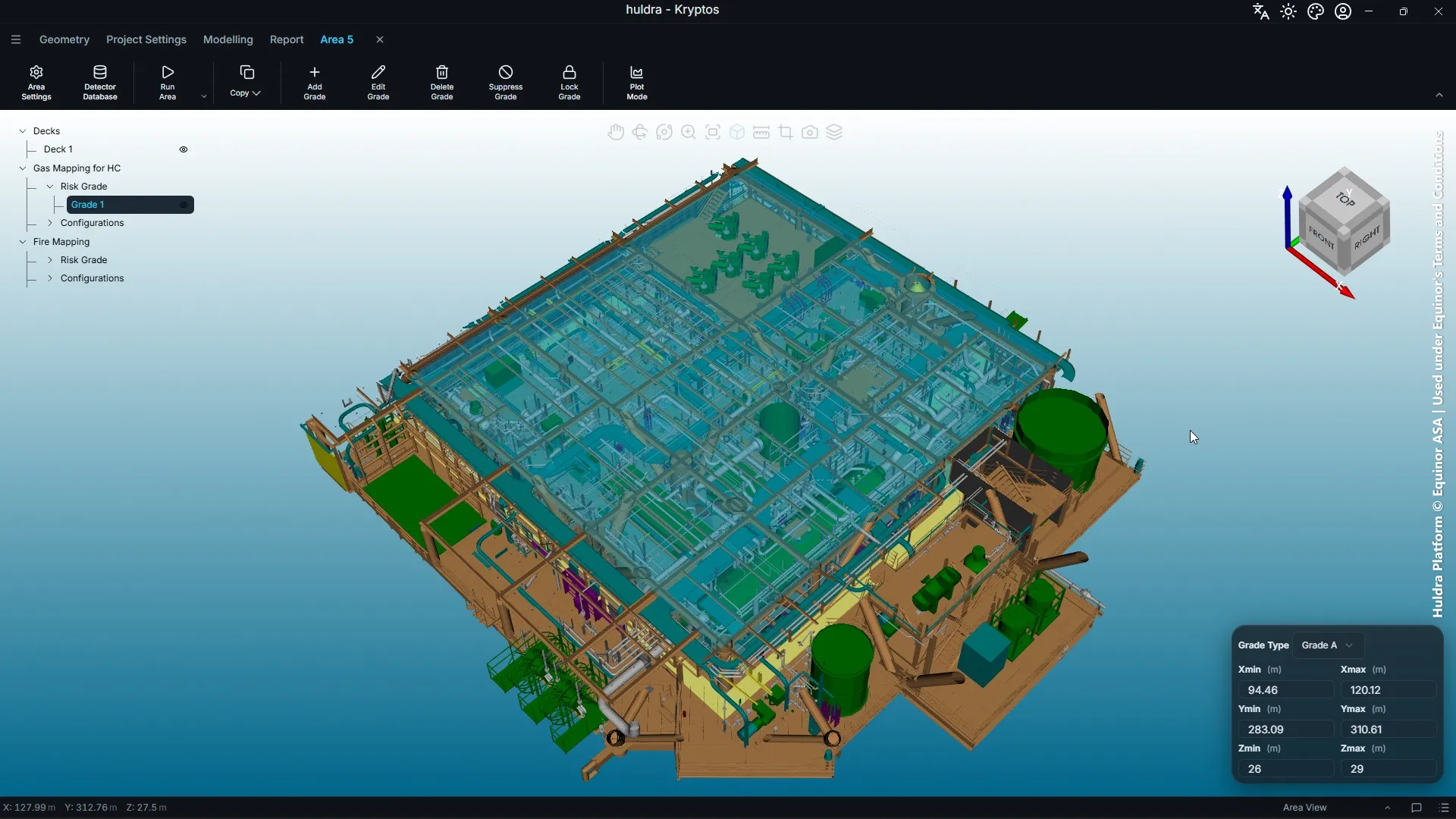
The blue highlighted part is the risk grade we used: a box of 25 × 27 × 3 m.
Step 4: Draw the deck
Kryptos only places detectors on decks: floors, platforms and walkways where a detector can be mounted. Detector heights are measured from the deck, so the deck also sets how high each detector sits.
- Select Decks in the area tree and click Add Deck.
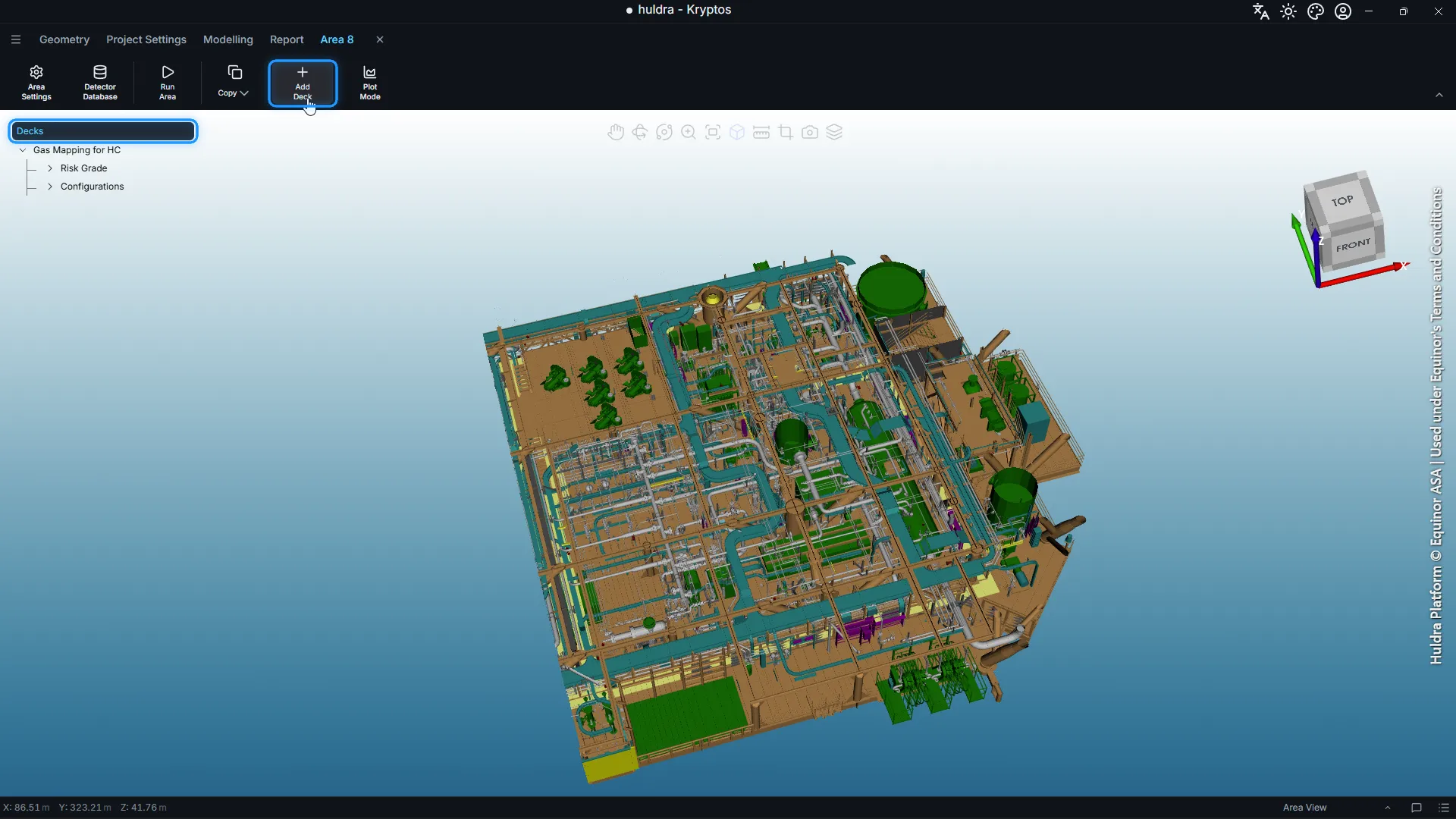
- Enter the Z Level of the floor, pick a shape and click Draw Deck.
- Draw the deck in the 3D view and click Complete.
An area without a deck cannot be optimised, because there is nowhere to put the detectors.
Step 5: Set the targets in Project Settings
Open the Project Settings tab. These settings apply to every area in the project.
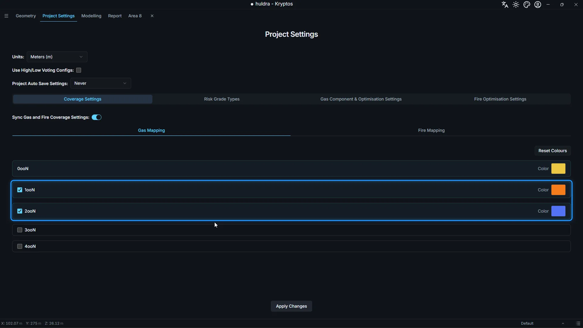
Coverage Settings
Tick the voting levels you need. We used 1ooN (at least one detector sees the gas) and 2ooN (at least two see it). Two detectors agreeing is what usually starts an automatic shutdown, so 2ooN is the number most studies care about.
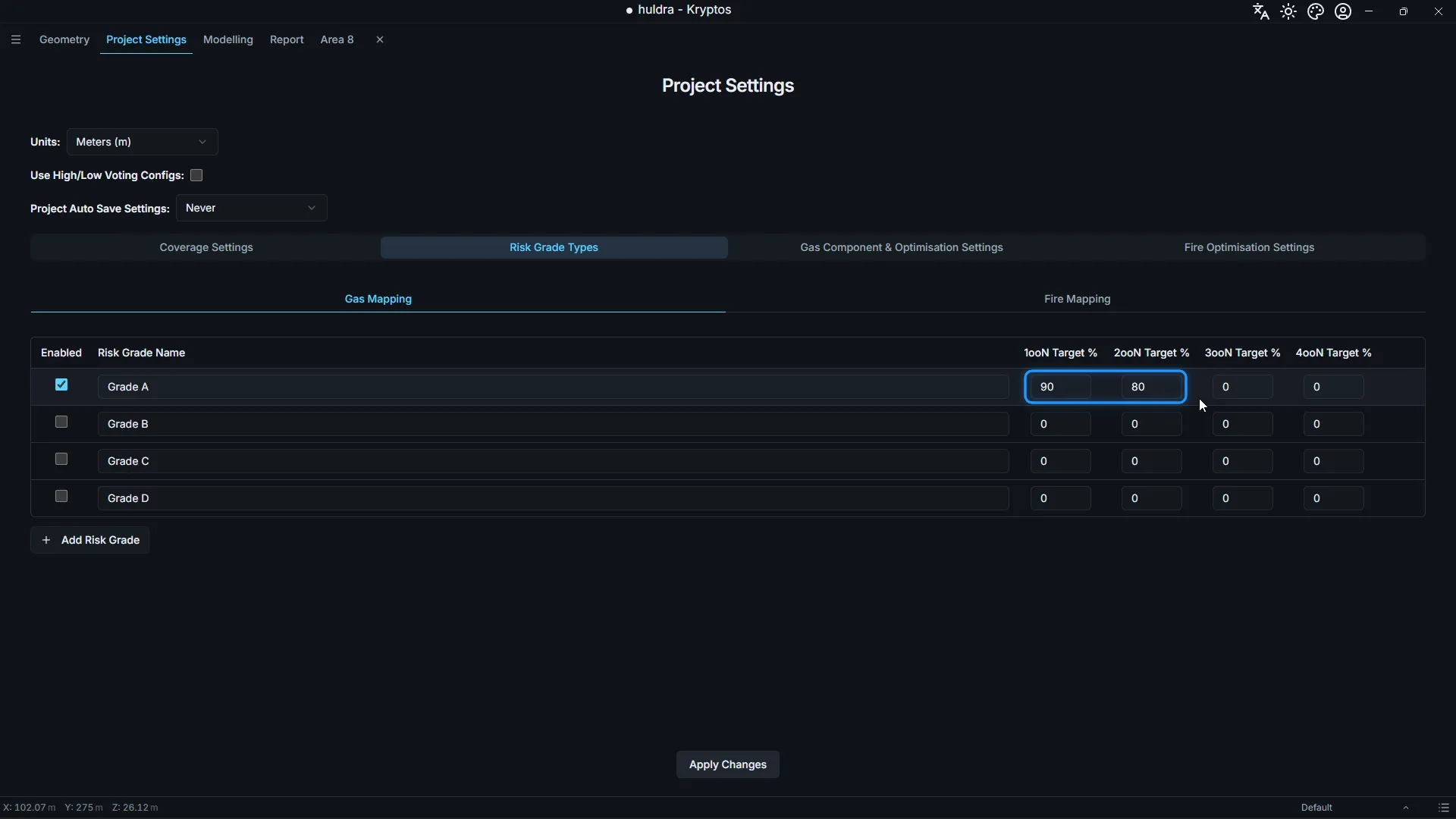
Risk Grade Types
Enter the target coverage for each grade at each voting level. This is the number the optimiser works towards. We set Grade A to 90% at 1ooN and 80% at 2ooN. A target of 0% asks for nothing.
Gas Component & Optimisation Settings
For each gas, choose whether open path detectors may be used (OPGD Available?) and set the height range above the deck for open path detectors (OPGD) and point detectors (PGD).
For run 1, we allowed open path detectors at 2 m to 5 m and point detectors at 0.5 m to 1.5 m.
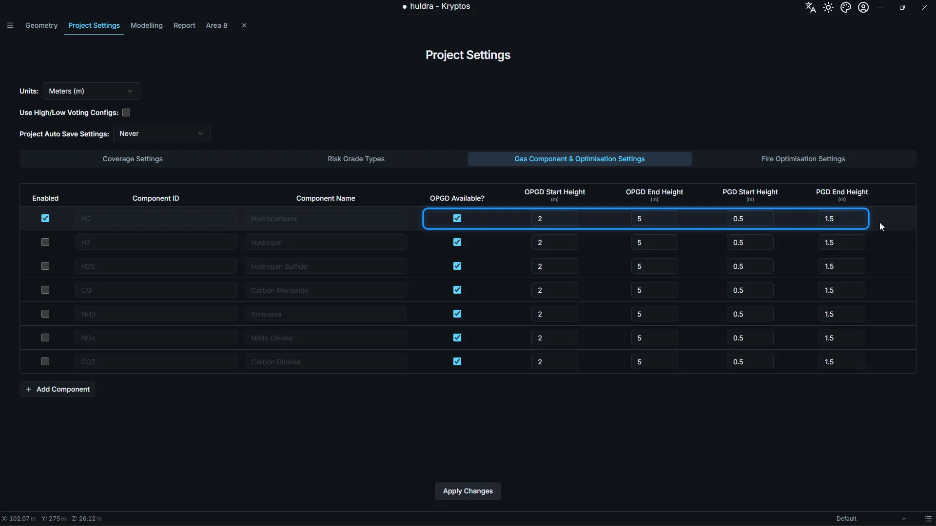
Heights are measured from the deck, not from the ground. If the deck is at 24.5 m and a detector goes 1 m above it, enter 1, not 25.5.
Click Apply Changes.
Step 6: Run the area
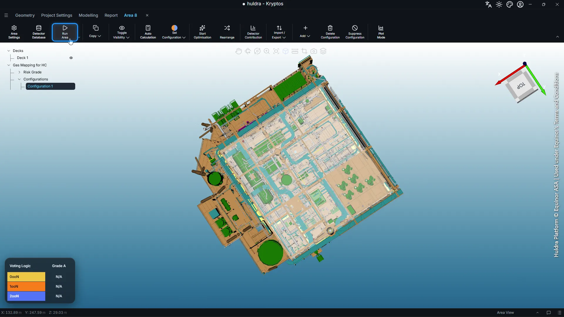
Open the area again and click Run Area. This works out where gas can reach on the deck and which spots a detector can see from. The optimiser needs it before it starts.
Step 7: Start the optimisation
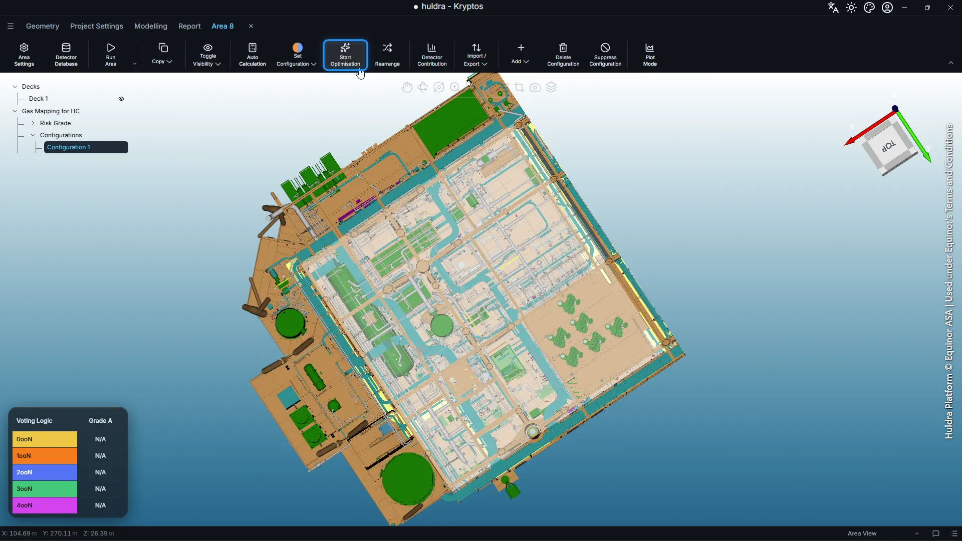
With the empty Configuration 1 selected, click Start Optimisation.
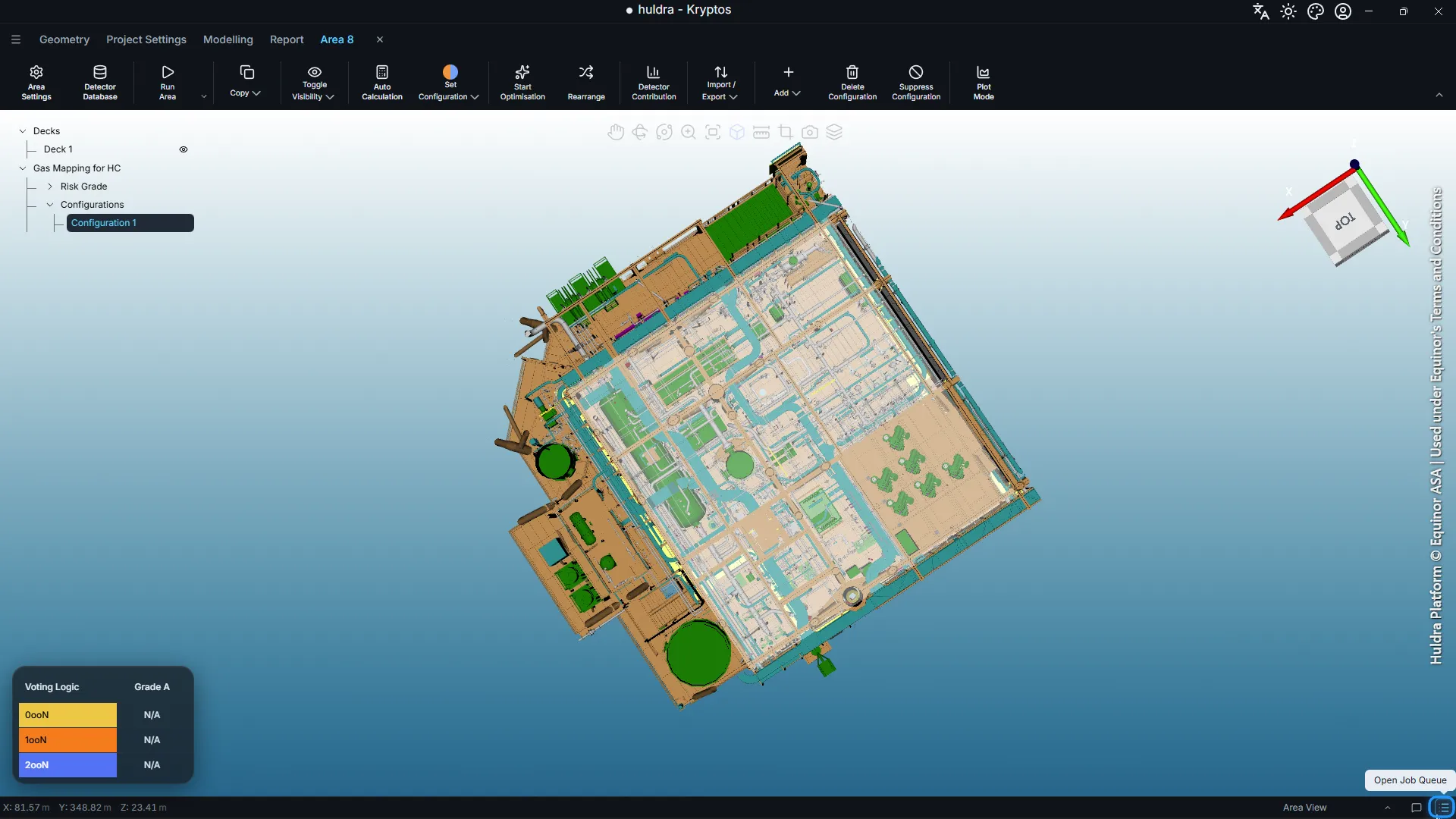
The run goes into the Job Queue. Open it from the icon at the bottom right of the window.
Each run shows as a card with its progress. Click the card to watch a live chart: each bar is the coverage so far at one voting level, and the dashed line is its target.
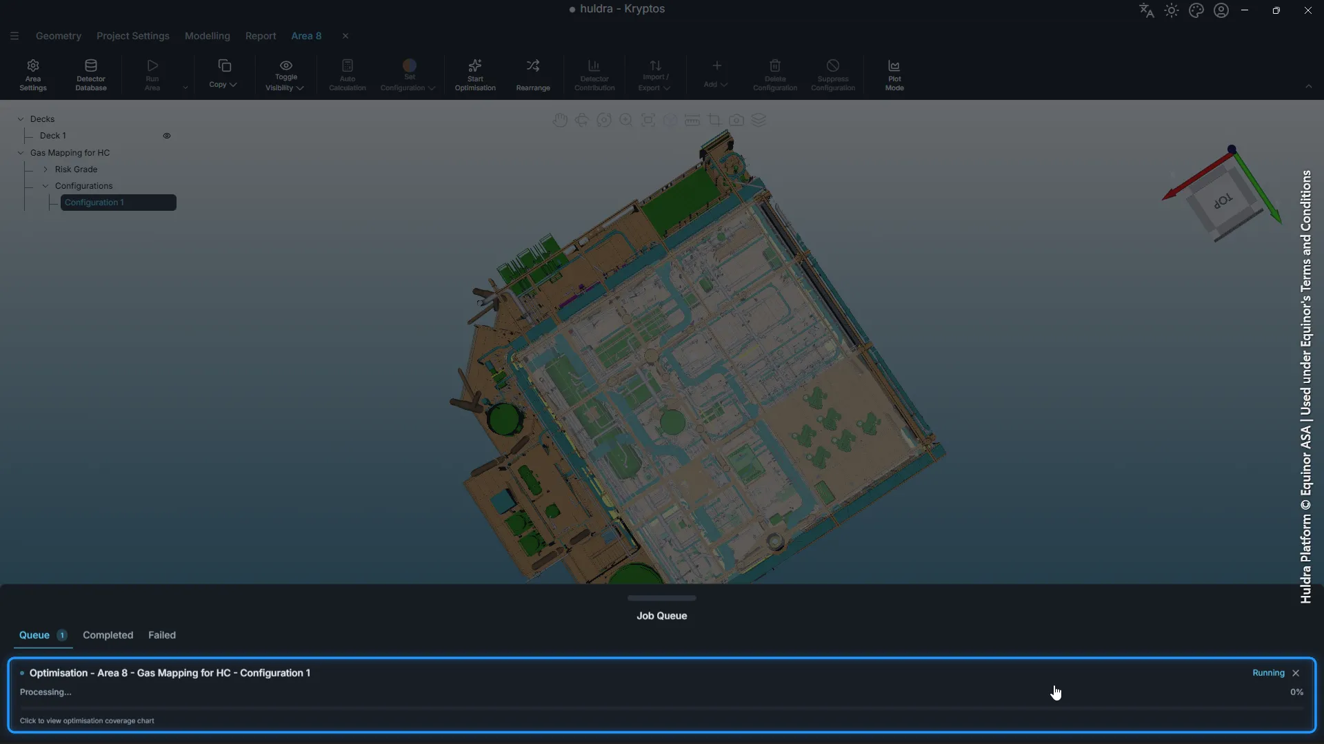
You can keep working while it runs, for example drawing the grades of the next area.
Tip: If some detectors must stay where they are, add them to the configuration first and lock them. Kryptos counts their coverage and places the new detectors around them.
Step 8: Check the result
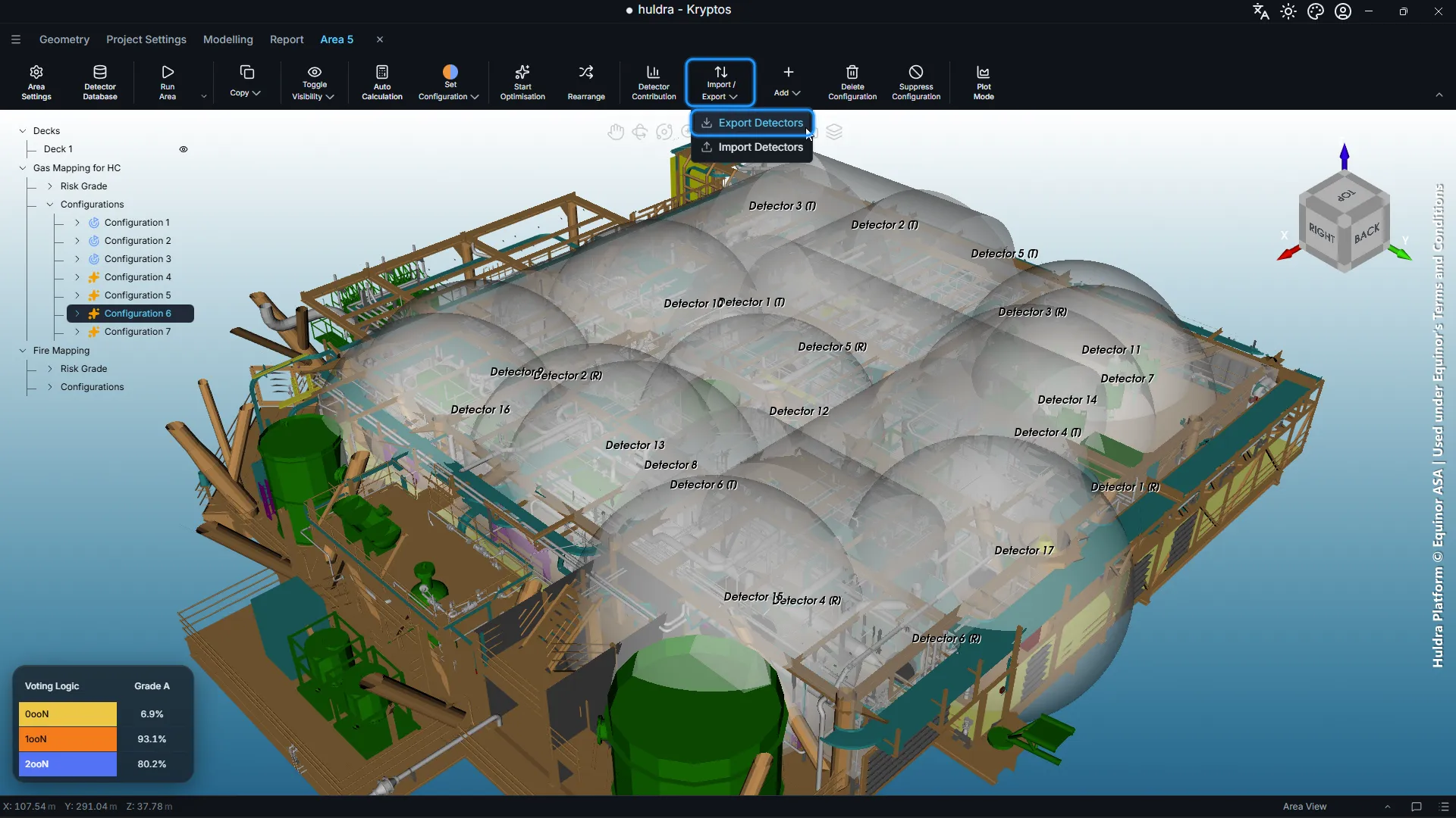
When the run finishes, the detectors appear in the 3D view and in the tree under the configuration. The Voting Logic panel at the bottom left shows the coverage of each grade at each voting level.
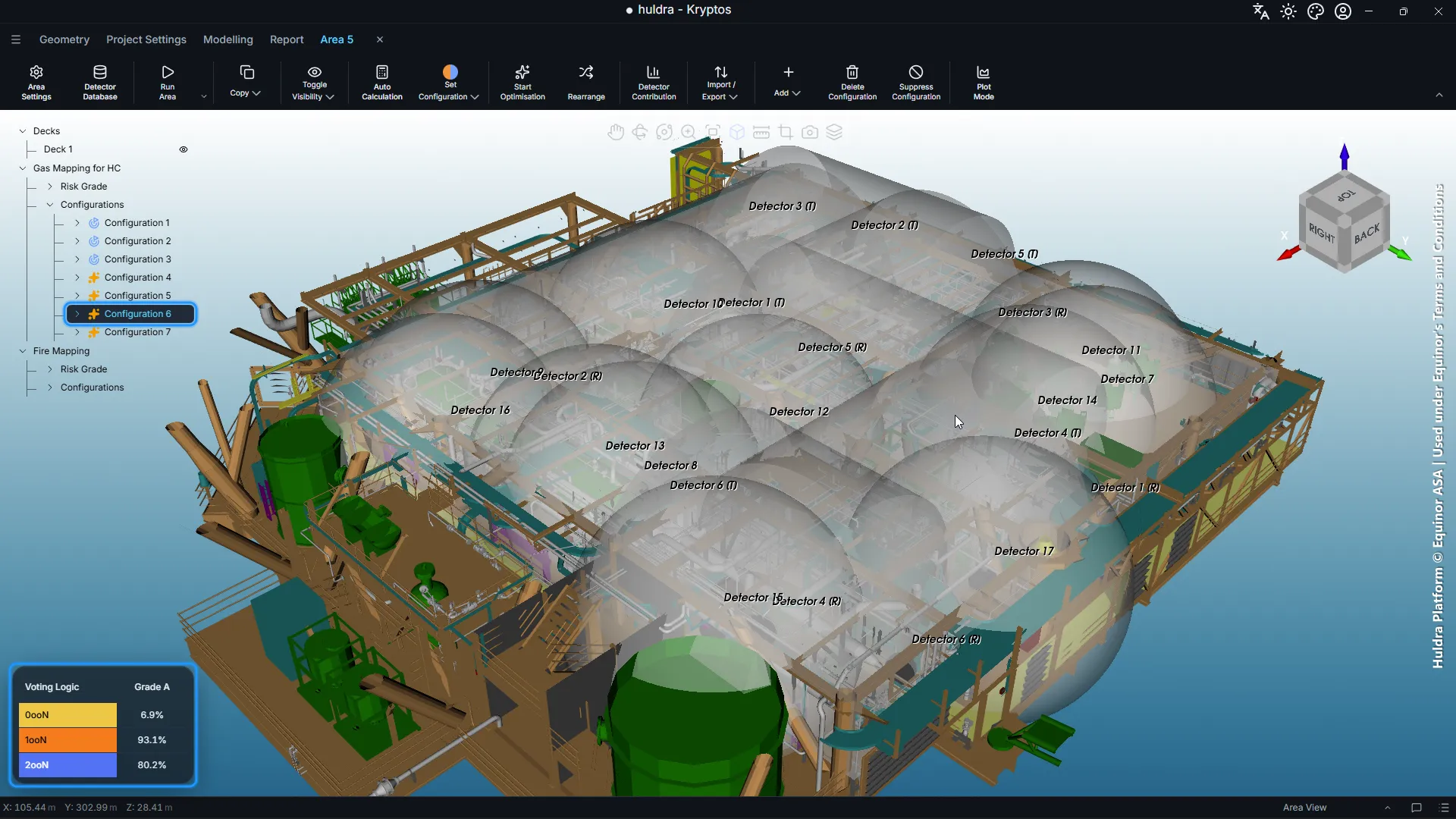
Run 1 placed 17 detectors, 6 open path and 11 point, and reached 93.1% at 1ooN and 80.2% at 2ooN, above both targets. Only 6.9% of the deck (0ooN) is seen by no detector at all.
Each open path detector is a beam between a transmitter, marked (T), and a receiver, marked (R). The other detectors are point detectors, each drawn with the 10 m gas cloud it can find. This deck is too crowded for long clear beams, so only 6 open path detectors fit and the optimiser filled in the rest with point detectors.
Step 9: Generate the plot
The percentages tell you how much is covered. A plot shows you where, so you can see which corners are weak and check that the layout makes sense on the real deck.
- Select the configuration and click Plot Mode.
- Leave Plot Type on 3D Plot and click Generate Plot.
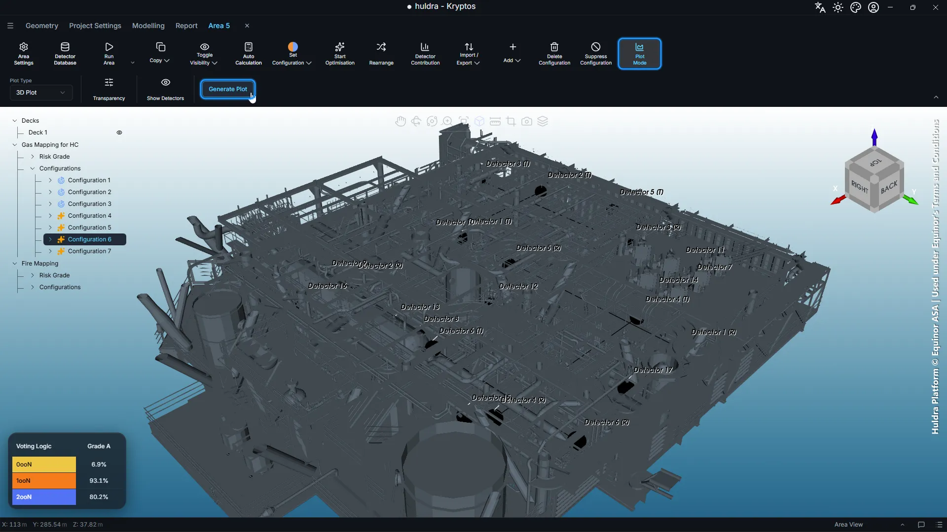
The covered space fills in, coloured by voting level. The legend at the bottom right gives the colours: here, blue is 2ooN, orange is 1ooN and yellow is 0ooN.
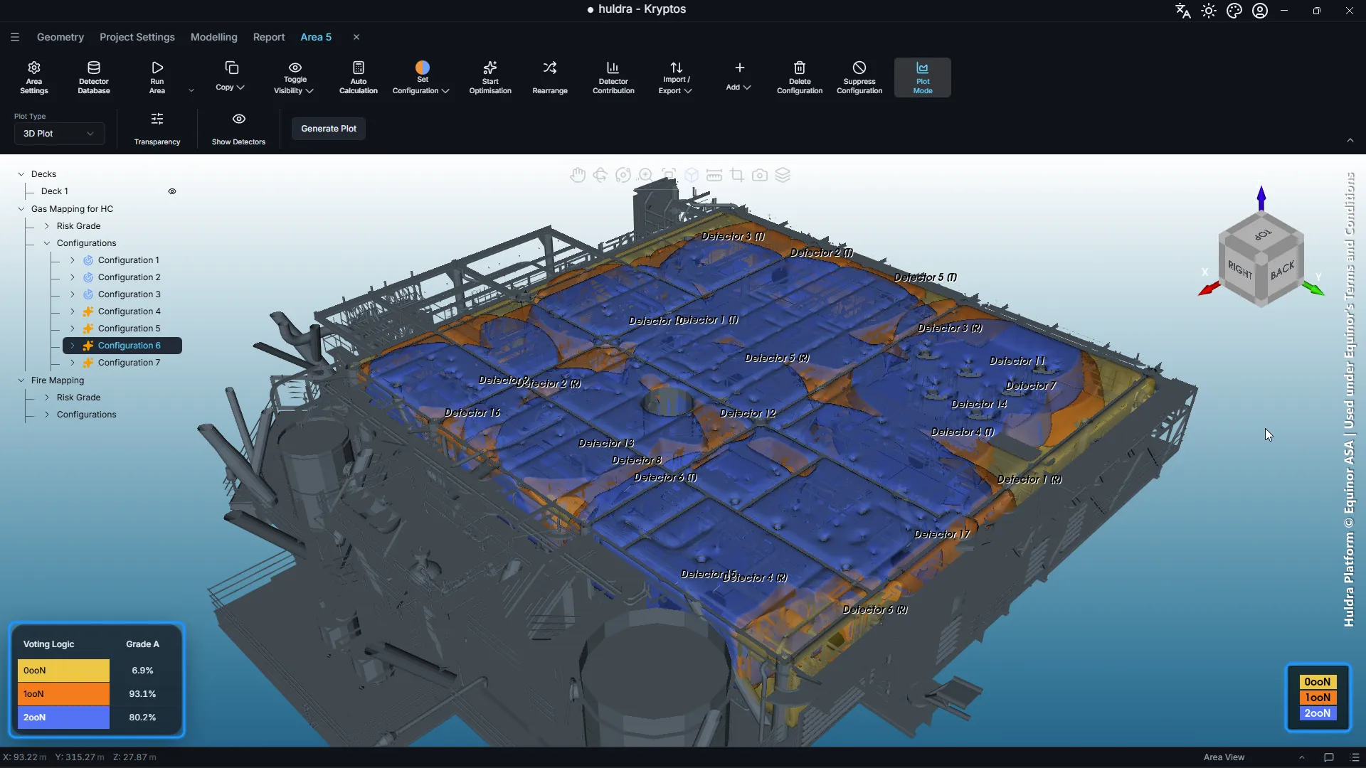
On the cellar deck, most of the deck is blue, so at least two detectors see a gas cloud there. The orange patches along the edges and between equipment are seen by one detector only. If those spots hold equipment that leaks easily, that is where to add a detector or move one. Anything yellow is seen by no detector at all.
A few more options in the same row:
- Transparency makes the plot more see-through, so you can see the equipment under it.
- Show Detectors shows or hides the detectors and their labels.
- Plot Type set to Slice Plot gives flat cuts through the area instead. Drag the slider, or press play, to move the cut through the deck.
Step 10: Export the detectors
To hand the layout on, for example to the team placing detectors in the 3D model or on the drawings, export it to Excel.
- Select the configuration.
- Click Import / Export, then Export Detectors.
- Choose where to save the file. Kryptos names it after the configuration, such as Configuration 6_detectors.xlsx.
For gas detectors, the workbook has two sheets:
| Sheet | Columns |
|---|---|
| Open Path Detectors | Detector Name, Component, X1, Y1, Z1 (one end), X2, Y2, Z2 (the other end) |
| Point Detectors | Detector Name, Component, X, Y, Z |
Every position is in project coordinates, so it matches the plant model. For run 1, the Open Path Detectors sheet lists each beam with both of its ends, and the Point Detectors sheet lists the rest.
The same file works the other way round. Change a position in Excel, or fill in detectors from another source, then use Import Detectors in the same menu to bring them into a configuration.
Run 2: point detectors only
Some projects use point detectors only, for example to avoid keeping open path beams lined up. To see what that costs, we ran the same deck again with open path detectors switched off.
- In Project Settings, open Gas Component & Optimisation Settings.
- Untick OPGD Available? for HC. The open path heights grey out.
- Click Apply Changes, add a new empty configuration to the area, and click Start Optimisation again.
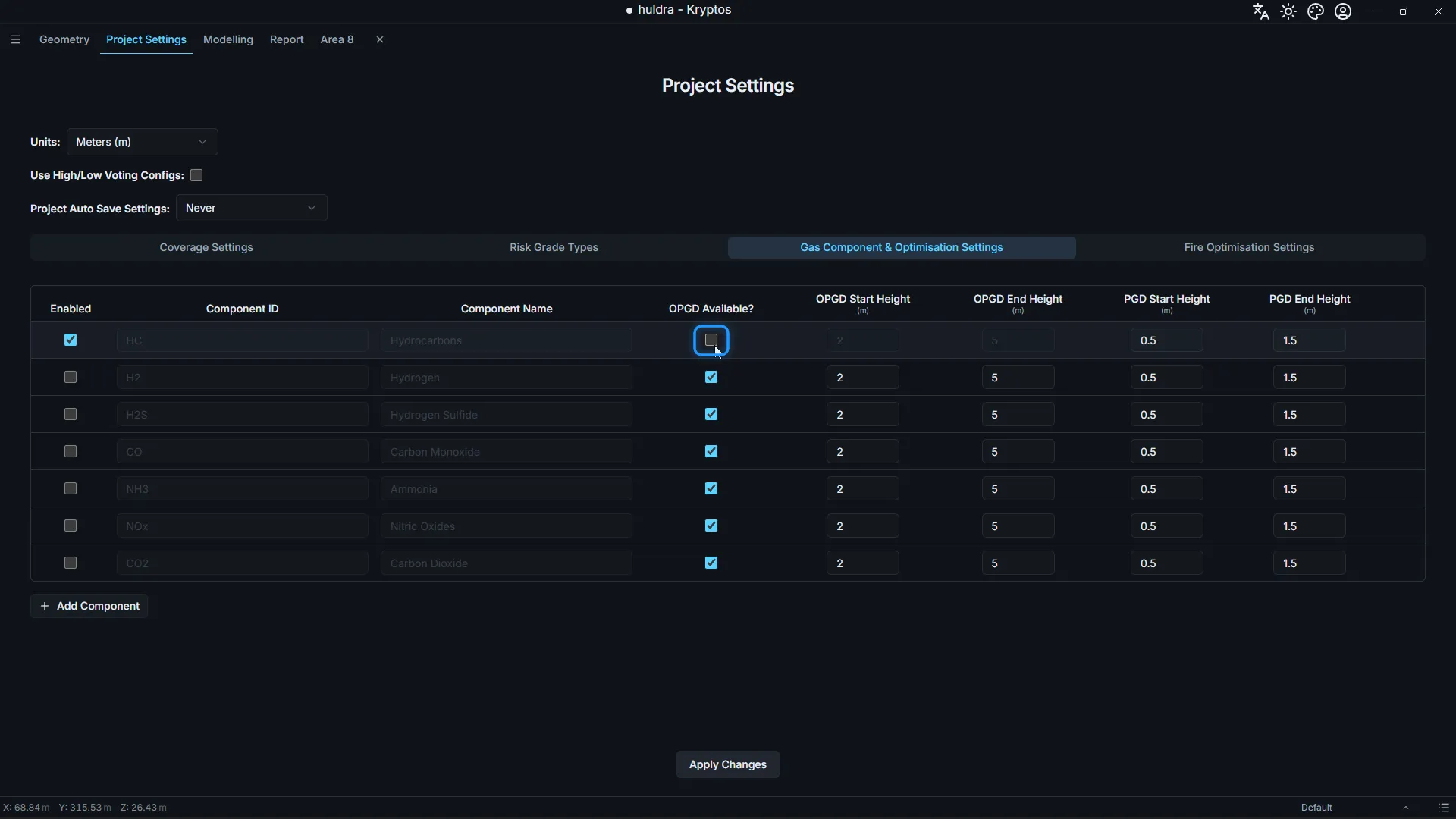
Everything else stayed the same: the same deck, the same 10 m gas cloud, and the same 90% and 80% targets. Run 2 reached 94.1% at 1ooN and 80.1% at 2ooN.
How fast was it?
We timed both runs from clicking Start Optimisation to the run finishing in the Job Queue.
| Run 1 | Run 2 | |
|---|---|---|
| Detectors allowed | Open path and point | Point only |
| Area | 38 × 40 × 5 m | 38 × 40 × 5 m |
| Gas cloud | 10 m | 10 m |
| Targets (1ooN / 2ooN) | 90% / 80% | 90% / 80% |
| Detectors placed | 17 (6 open path, 11 point) | 22 (all point) |
| Coverage (1ooN / 2ooN) | 93.1% / 80.2% | 94.1% / 80.1% |
| Total time | 1 min 8 s (68 s) | 2 min 39 s (159 s) |
| Time to find optimised position per detector | 4.0 s | 7.2 s |
Measured on a laptop with an Intel Core i7, 16 GB of RAM and 8 GB of graphics memory.
What the numbers show:
- Run 1 finished in just over a minute. That is a full process deck, from an empty configuration to a layout that beats both targets, in 68 seconds.
- Open path detectors saved 5 detectors. The deck is crowded, so only 6 beams had a clear line across it, but they were enough to bring the count down from 22 point detectors to 17 detectors in total.
- Run 2 took more than twice as long. With open path detectors switched off, the run took 159 seconds instead of 68, and it placed more detectors.
- Each detector took only a few seconds. Finding the optimised position for each detector took about 4 to 7 seconds in both runs, so a bigger layout costs seconds per detector, not hours.
- Comparing options is cheap. Answering “what if we only use point detectors?” took one tick box and under three minutes. You can try a different cloud size, target or height range the same way, and keep each result as its own configuration to compare.
Your times depend on the size of the area, the gas cloud size and your computer.
What’s next
The same steps work for fire detectors, with a few extra settings for each detector’s view. See Fire detectors auto-placed and aimed by Kryptos on a real offshore deck, in 63 seconds.
Credits and acknowledgements
The plant model in this post is the Huldra platform, © Equinor ASA, used under Equinor’s Terms and Conditions. Our thanks to Equinor for making the Huldra data openly available, which lets us show Kryptos working on a real offshore platform.
Every screenshot and video that shows the model carries this credit. Equinor has not reviewed or endorsed this post or Kryptos.
Model credit: Huldra Platform © Equinor ASA | Used under Equinor's Terms and Conditions